Geotimes

Feature
Precision Agriculture:
Changing the Face of Farming
Doug Rickman, J.C. Luvall, Joey Shaw, Paul Mask, David Kissel
and Dana Sullivan
Sidebar: Defining
images
A description of agriculture is one of superlatives. Its economic impact, extent
of land use, and environmental and social significance are all of the first magnitude.
The U.S. Department of Agriculture (USDA) estimates there are 2.1 million farms
in the United States, using 941 million acres (about 1.5 million square kilometers)
of land, with production worth $200 billion a year. Just as manufacturing has
changed radically in the last two centuries, farming has also changed. The classic
picture of the farmer — one of bucolic simplicity — is wildly out of
date. Costs, technology and economies of scale have driven commercial farms around
the world to change. And remote sensing is beginning to play a large role.
American farmers annually spend $23 billion for fertilizer, chemicals and seeds
and $9 billion for energy. A harvester, which costs approximately $125,000, cuts
a swath 5 meters wide with each pass, measuring the amount of grain and its moisture
content on the fly. Juggling spot market prices versus current delivery contracts
versus available storage in grain elevators on the farm and at the co-op, the
farmer must balance complex business factors even in the middle of the harvest.
In the United States, a farm operator must now manage a square mile or more to
be viable. The size of an individual production unit — a field — now
measures hundreds of meters on a side. Typically, all portions of that unit are
treated the same. Crop varieties, seed density, soil preparation, fertilizers,
herbicides, insecticides and fungicides are uniformly applied. But plants respond
to major environmental and soil variables that vary on fine scales. The resulting
mismatch between the uniformity of crop treatments and the uniqueness of individual
plants’ physiological responses means some portion of the farmer’s costs
are going to be wasted.
Precision agriculture integrates a suite of technologies that retain the benefits
of large-scale mechanization, which is essential to large fields, but recognizes
local variation. By using satellite data to determine soil conditions and plant
development, these technologies can lower the production cost by fine-tuning seeding,
fertilizer, chemical and water use, and potentially increasing production and
lowering costs — all benefiting the farmer. In turn, precision agriculture
may have significant impacts far beyond the individual farm. Pollution, for example,
is a common problem stemming from agricultural practices. Excess agricultural
chemicals from a field must go somewhere, and somewhere frequently means the common
environment. Precision agriculture can reduce the volume of those extra chemicals.
Application of precision agriculture has at its heart two spatial requirements:
concurrent knowledge of where the farm equipment is as it moves across a field
and the value of one or more variables as a function of position within the field.
These two requirements each contain a “where” and a “what.”
The spatial precision needed for “where” varies from a few meters to
a few centimeters, but GPS, computer circuits and electronic systems can now satisfy
that. In fact, using real-time kinematic GPS, it is practical to automatically
guide huge farm machines to stay along a track hundreds of meters long with only
centimeter-scale deviations. The second requirement, the “what,” is
where remote sensing comes into the picture.
Our NASA team of geoscientists is working with the Advanced Thermal and Land Applications
Sensor (ATLAS) remote-sensing instrument flown on the NASA Stennis Lear jet to
understand the driving thermal processes in crops and to fine-tune precision agriculture
capabilities.
Meeting the challenge
Remote sensing has had agricultural applications from the earliest days. In
turn, agriculture has helped drive the design of major remote-sensing instruments.
For example, the spectral bands, spatial resolution and orbital elements of
the original Multi-Spectral Scanner on the Earth Resources Technology Satellite,
launched in 1972, were influenced by field size, field spectrometer data on
crop leaf and soil reflectance, and crop life cycles.
To a large extent our work has grown out of the remote-sensing technology and
conceptual framework developed by geologists. For example the drive to look
at the physics of reflectance and atmospheric corrections is rooted in work
done in the early 1980s by the U.S. Geological Survey and NASA. Our work on
emissivity and thermal behavior of plants pulls on research done using the Thermal
Infrared Multispectral Scanner, an instrument originally conceived for geologic
applications. Even our ability to geometrically map the airborne imagery onto
the globe was explicitly developed because of the need to map sediment flow
patterns along the coast of Louisiana.
This influence has continued and can be found in the Thematic Mapper and a number
of other sensors. Agriculture also has been the focus of major research programs,
for example the Agriculture and Resources Inventory Surveys Through Aerospace
Remote Sensing (AgRISTARS) program, funded by USDA and NASA from 1974 into the
early 1980s. Academic, government and corporate researchers have sought to apply
remote sensing to a wide range of agricultural challenges, such as detecting
drought, controlling fungus, diseases and insects, forecasting production, and
determining acreage per crop.
But utility has not been easy to achieve because of numerous difficulties, both
in logistics and basic physics. Clouds are one practical problem. Long intervals
between satellite passes can easily miss critical growth stages. Physically,
the reflectivity of one green plant looks very much like that of any other green
plant. Multiple reflectance sources, such as soil, shadow, moisture and plant
growth, each with a range of properties, can combine in multiple ways to give
non-unique signals. And many of the phenomena are not independent. For example,
volumetric variation of the sand percentage changes the water availability profile
with time, which affects plant growth under some but not all rainfall histories.
Changing the amount of sand also mandates changes in other soil constituents,
which in turn also have other impacts.
These problems frequently cause errors. For example, when processing data sets
that cover 100 kilometers or more on a side, it is common to have the analytical
tools erroneously determine that there is corn in the middle of wheat fields
and wheat in the middle of a city. One of the laboratory directors responsible
for some of the AgRISTARS work, Wayne Mooneyhan, commented, “we were more
successful estimating wheat yields by monitoring the Soviet lake levels than
by actually monitoring the fields.” In that case, the amount of water used
for irrigation was a better estimator than direct observation of the fields.
For many applications of remote sensing in agriculture, the solution to such
problems has been the use of statistical abstractions, which provide a simple
number representing some feature of a large area, rather than identifying exactly
where corn or soybeans are located, for example. Because large areas are necessary
for this methodology to be valid, the agricultural consumer of remote sensing
tends to have interests far broader than a single field or even a county. Therefore,
government agencies, such as state and USDA agricultural statistical services,
are typical users.
But precision agriculture is not about an abstract measurement or characterization.
It is about specific values at exact locations and helping the individual farmer.
This change in focus requires a recognition of why the earlier work has had
limited impact at the finer scale. We have identified several areas as high
priority for acquiring more data, including acquisition conditions (cloud cover,
time of day, soil condition, etc.), the nature of the signal (atmospheric effects,
improper models, erroneous assumptions, etc.), and cost and applicability to
the customer.
We have been working to meet these challenges, several of which can be solved
simply with the right engineering choices. For example, using an airborne sensor,
we have addressed acquisition conditions and timeliness. Other challenges are
less straightforward, such as cost, which is a difficult concept, as it depends
on the market structure. Simple estimates range over several orders of magnitude.
Therefore, we must defer tackling these economic challenges until we have answers
to more technical questions.
Our team has approached the other problems by integrating agronomy, plant physiology
and soil science with a physics-driven framework and attention to thermodynamics.
Our current results, which are by no means complete, are extremely encouraging.
We have shown that the temperature of a crop can be highly correlated with its
yield. The plant can be considered as an engine for evaporating water, and a
relationship exists between how much water is evaporated and the productivity
of the plant. We also have seen that multi-band thermal imagery is sensitive
to soil conditions.
Matching energy and yield
The dominant “design criteria” for land plants is to shed the majority
of all incoming radiation. Of the total incoming energy, a plant uses about
1 percent for photosynthesis. If the plant does not shed the remaining energy,
it will quickly heat up until the biochemistry involved fails and the plant
dies. About 2 percent of the incoming energy is used to heat the mass of the
plant. Six percent is used to heat the air, and some 10 percent of the incoming
energy is rejected through reflection. Approximately 43 percent of the energy
is converted to heat and radiated to the sky in thermal wavelengths. Virtually
all the remaining energy, 48 percent, is used to evaporate water. Thus a plant
is like an engine whose major function is to convert water into water vapor
using solar radiation.
The water used for cooling is obtained by the roots, moved to the leaf and then
evaporates. The plant must also move the dissolved gases, carbon dioxide and
oxygen, and various biochemicals involved in photosynthesis. With the efficiency
of a good engineering design, evolution has given plants a single mechanism
for both cooling and chemical transport. This mechanism — evapotranspiration
— intrinsically ties the thermodynamic behavior of a plant dealing with
incoming radiation to its basic biochemistry.
Anything that decreases evapotranspiration will decrease the plant’s synthesis
of chemicals. As evapotranspiration decreases, that portion of the energy not
used to evaporate water must go into other parts of the energy equation. Therefore,
if we can say something about the energy balance for a plant, we likely can
say something about the productivity of the plant. And we can then apply these
concepts to an entire crop.
A single field is made up of plants that are genetically very similar and of
the same age. Thus even some minor factors, which have been ignored in the above
energy balance discussion, tend to be suppressed. Cooler areas of a given field,
we believe, will tend to be more productive, and our results substantiate this.
In properly acquired imagery, high-yield areas are noticeably cooler. In fact
it is possible to get very good correlations between remote-sensing imagery
and yield from images taken a long time before harvest. And these correlations
are markedly higher than can be achieved with other approaches.
Making a difference
We must resolve many challenges before this relatively simple relationship
between temperature and yield becomes a generic, commercially viable tool (see
sidebar and images). The approach cannot rest solely on the correlation between
temperature and yield. Still, we have learned much in the last few years and
believe our integration of geologic remote sensing with other fields of expertise
was a wise investment. Clearly none of the specialties alone could develop,
let alone test, the basic approach we are now finding so powerful. This is the
path that will ultimately produce information needed by farmers. But we also
recognize how small a portion of the total problem has been solved. Having developed
the basic logic, built prototype tools and performed initial tests, we can see
everything else that remains to be done. And problems, both scientific and practical,
are everywhere.
At times the list of problems seems endless. We have not established sensitivities.
We have not robustly segregated the contributions of crop residue, soil moisture,
shadows, plant and soil to the energy leaving the surface. What we do is extremely
expensive and difficult. It is experimental in methodology and uses research-oriented
tools. We are constantly alert to the practicality of moving our results into
commercial applications. We know another airborne instrument will have to be
available. Atmospheric parameters will have to be measured automatically. The
software will have to be rewritten for speed.
But the potential is also enormous. Agriculture is a huge portion of our economy.
Just a 1 percent increase in efficiency is a $2 billion change. We all depend
on farmers, literally, for the bread we eat. No other human activity has an
impact on land that matches that of farming. If application of precision agriculture
can help farmers better manage their land, we all may benefit.
Defining
images
Before precision agriculture can reach its potential, researchers must
resolve several challenges, both mechanically and quantitatively. Several
examples follow. Images and text provided by Doug Rickman.
UNITS Ordinary
remote-sensing data are not in reproducible units. The basic measurements
are on an ordinal scale of varying significance; in other words values
are simply “brighter” or “darker.”
To overcome this challenge, our long-term goal is to convert all the remote-sensing
measurements into physically meaningful units, and to be able to fully
model the radiation entering and leaving each pixel of the data set. Doing
this in a manner that is driven by first principles requires detailed,
site-specific knowledge of the atmosphere, modeling of radiative transfer
in the atmosphere and an active calibration source within the sensor.
Although the process is long, complex and demanding, it is now possible
to explore quantifiable relationships, such as the sensitivity of the
remote-sensing data to leaf nitrogen content, and to hope that the results
can be applied generically.
Moving into calibrated measurements allows direct measurement of soil
chemistry. Emission from a material is a function of temperature and emissivity.
Emissivity is the ratio of energy emitted by a material compared to the
energy emitted by a “blackbody” (something that absorbs all
light) at the same temperature. For virtually all earth surface materials,
temperature is far more important than emissivity and therefore dominates
imagery made from thermal (7- to 13-micrometer wavelengths) spectral bands.
It also means imagery from multiple thermal bands is very highly correlated.
At Earth’s surface conditions, emissivity is nearly independent of
temperature and particle size — controlled by chemical properties.
Vegetation and water have essentially no spectral variation in these wavelengths,
but the silicate and carbonate bonds of many minerals do affect emissivity.
 By
making a color composite image, assigning different spectral bands to
each of the color guns of the display, an image is made in which anything
that is not gray has different emissivities in the disparate bands. In
these images, any color difference is due to changes in mineralogy alone.
In urban areas, as seen at left in Salt Lake City, Utah, it is easy to
see changes in paving along highways and in airport runways. The emissivity
features of individual fields tend to be much less dramatic, as the original
features are much lower contrast and plowing has often diffused the boundaries
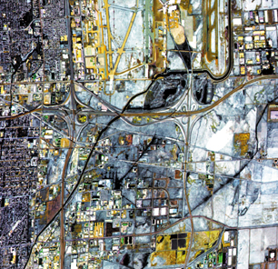
by mixing. By
making a color composite image, assigning different spectral bands to
each of the color guns of the display, an image is made in which anything
that is not gray has different emissivities in the disparate bands. In
these images, any color difference is due to changes in mineralogy alone.
In urban areas, as seen at left in Salt Lake City, Utah, it is easy to
see changes in paving along highways and in airport runways. The emissivity
features of individual fields tend to be much less dramatic, as the original
features are much lower contrast and plowing has often diffused the boundaries
by mixing.
This image is a color composite
of three thermal bands, which are dominated by temperature. In a color
composite, perfectly correlated values (i.e. similar temperatures) become
gray, and thermal band data correlation is extremely high. Any color variation
is due exclusively to differences in emissivity between bands. Note the
change in paving types within the airport and along the various roadways.
Data from the ATLAS sensor over Salt Lake City, Utah.
 But in
some cases, such as breaking up of soil crusts, the plowing can lead to
very striking features, because the soil crusts are made of oriented and
segregated size fractions, whose mineralogy is not the same as the average
composition of the parent soil. More usefully, with quantitative remote-sensing
measurements, it becomes practical to do mineralogical evaluations of
soils that are spatially separated by arbitrary distances, as seen in
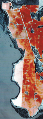
the image at right. But in
some cases, such as breaking up of soil crusts, the plowing can lead to
very striking features, because the soil crusts are made of oriented and
segregated size fractions, whose mineralogy is not the same as the average
composition of the parent soil. More usefully, with quantitative remote-sensing
measurements, it becomes practical to do mineralogical evaluations of
soils that are spatially separated by arbitrary distances, as seen in
the image at right.
Vegetation and water have nearly constant emissivities across the 7- to
13-micrometer spectral region, and the correlation makes them appear gray
in color composites of multiple thermal bands. The soils in these fields
are rich in quartz sands and clay minerals. Rainfall causes segregation
of the soil constituents. Plowing remixes them. The color variation in
the imagery is controlled by these factors. ATLAS data from Georgia.
 ALIASING
With high spatial resolution comes aliasing, where a non-existent pattern
appears because of sample spacing. The classic aliasing example is the
spinning propeller that appears to be moving in reverse of the true direction.
With crops, spatial sampling on the scale of a meter combines with the
row spacing to alias pseudo-rows that are tens of meters wide. To paraphrase
the old saw, in such cases you literally cannot see the crop for the rows. ALIASING
With high spatial resolution comes aliasing, where a non-existent pattern
appears because of sample spacing. The classic aliasing example is the
spinning propeller that appears to be moving in reverse of the true direction.
With crops, spatial sampling on the scale of a meter combines with the
row spacing to alias pseudo-rows that are tens of meters wide. To paraphrase
the old saw, in such cases you literally cannot see the crop for the rows.
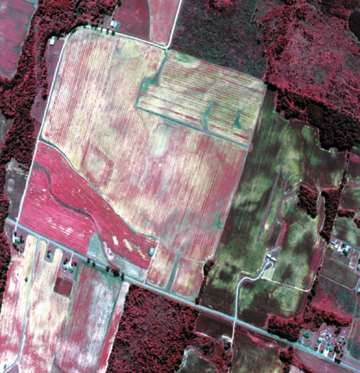
The apparent crop rows' spacing is larger than the roads and homes in
the image, which was taken with a nominal ground resolution of approximately
2 meters. The spacing of the rows is less.
Pictured at left is aliasing of crop rows into longer spatial wavelengths.
The apparent rows are false. Visual clues to this are seen by comparing
the apparent row spacing with the size of roads and homes. The imagery
was taken with a nominal ground resolution of approximately 2 meters.
The spacing of the rows is less.
Back to top
|
Rickman and Luvall are both
researchers in the Earth Science Department at the NASA Marshall Space Flight
Center. Shaw and Mask are researchers at Auburn University. Kissel is a professor
at the University of Georgia, and Sullivan works out of the Southeast Watershed
Research Laboratory, USDA-ARS.
Link:
"Satellite
precision farming," Geotimes News Note, August 2001
References:
Barnes, E.M., and Baker, M.G. (2000).
Multispectral data for mapping soil texture: possibilities and limitations.
Am. Soc. Agricultural Engineers, 16, 731-41.
Bryson, R. J. 2000. Remote sensing in agriculture. 26-28 June 2000. Royal Agricultural
College, Cirencester.
Environmental Remote Sensing Center. 2000. Earth observation satellites: future.
Available at http://www.ersc.wisc.edu/resources/EOSF.html.
Thomasson, J.A., Sui, R., Cox, M.S., and Al-Rajehy,
A. (2001). Soil reflectance sensing for determining soil properties in precision
agriculture. Am. Soc. Agricultural Engineers, 44, 1445-53.
Back to top
